Selected Course Projects
Category
Geometry Processing
Accelerate Marching Cubes
Simulate Sand as Fluids
Geometry Processing
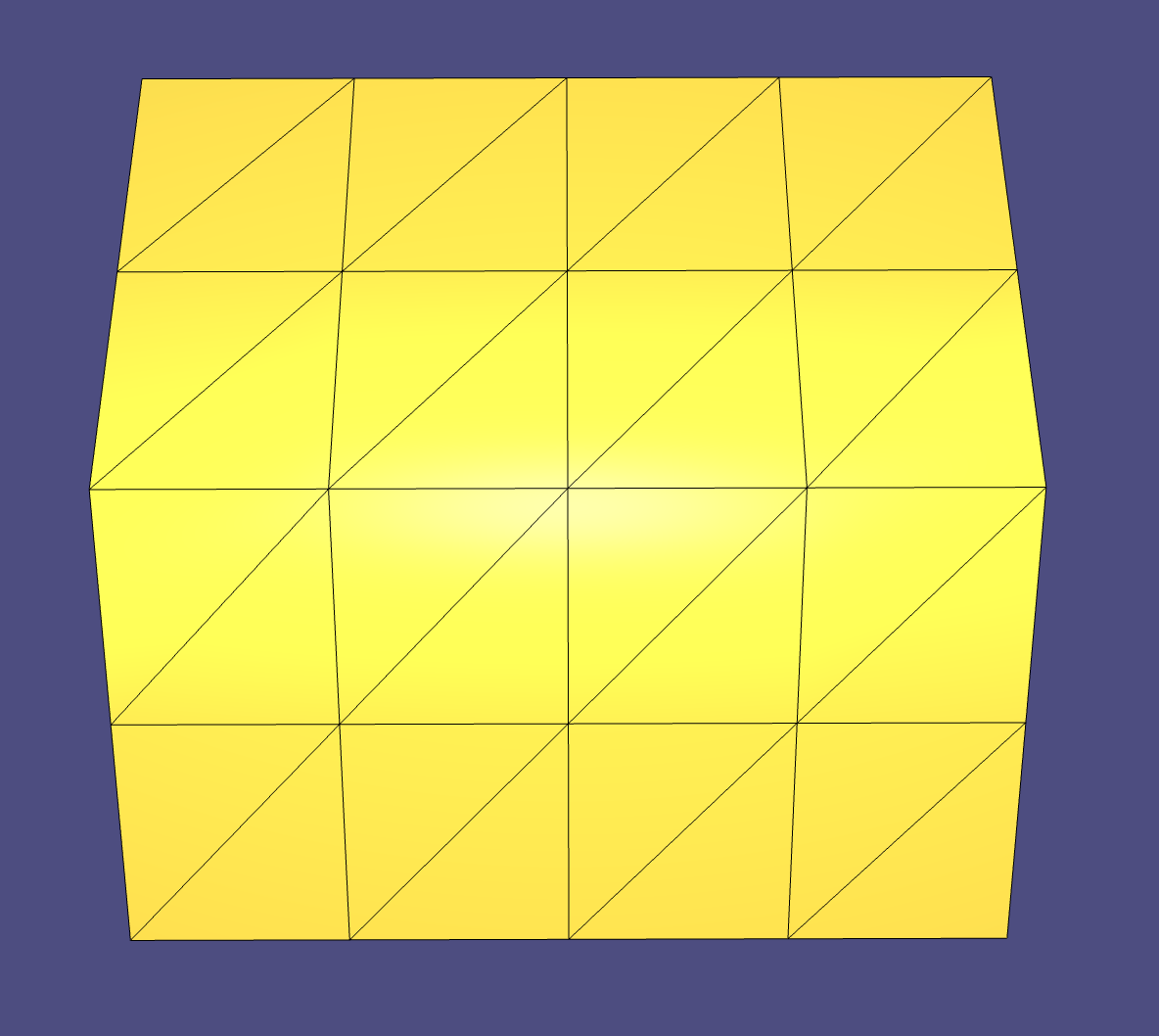
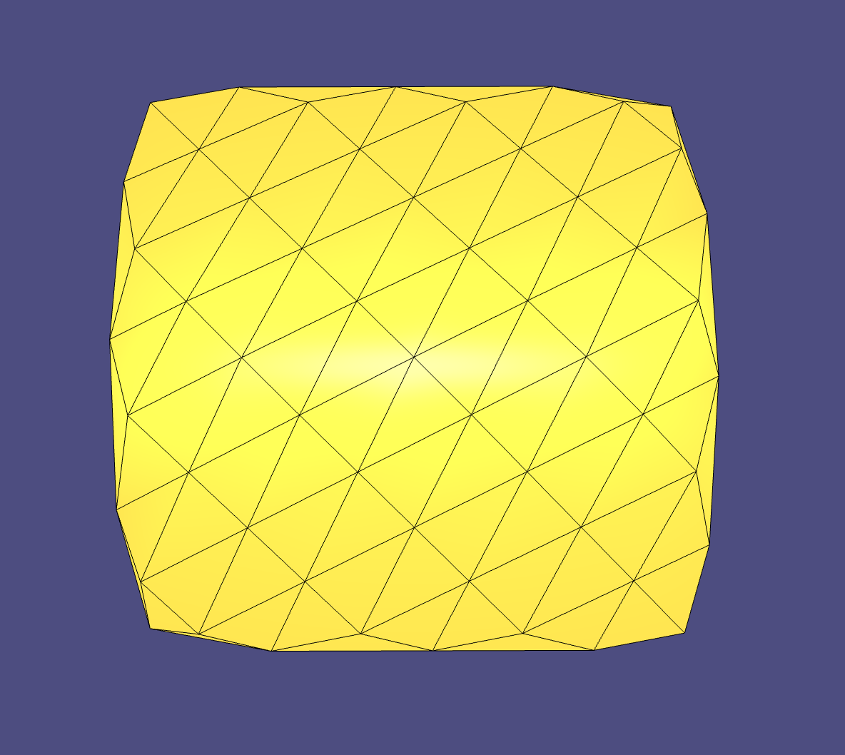
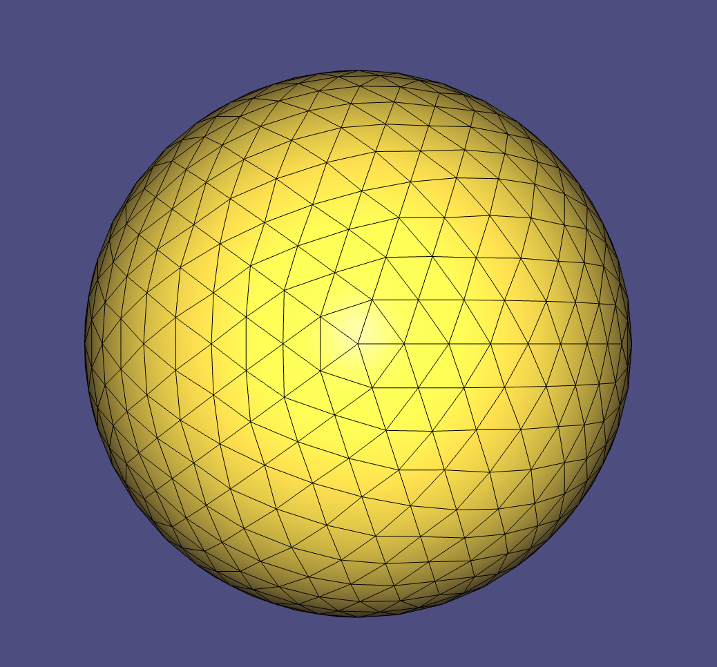
1. Mesh Subdivision
Implemented Sqrt(3) mesh subdivision scheme
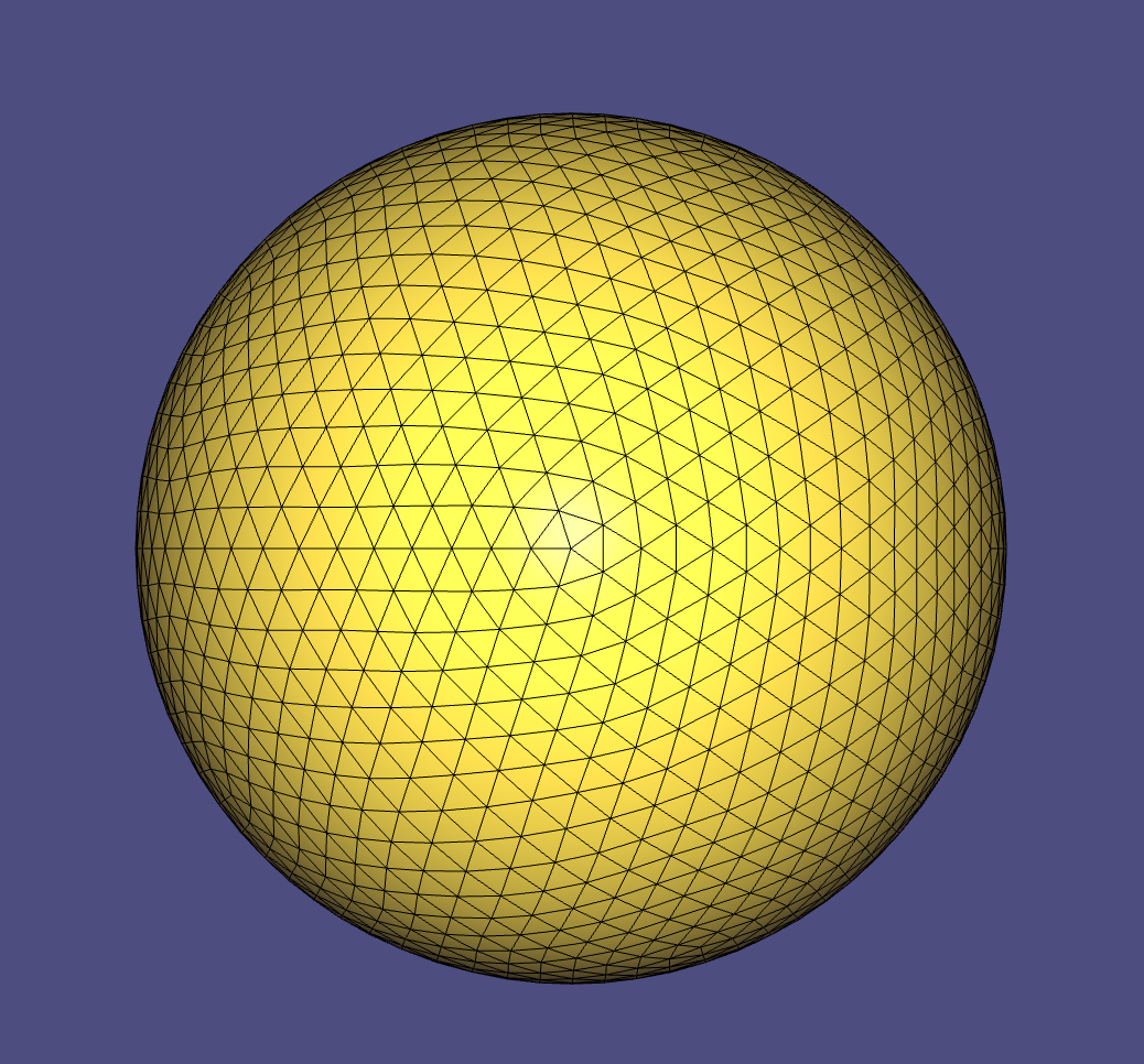
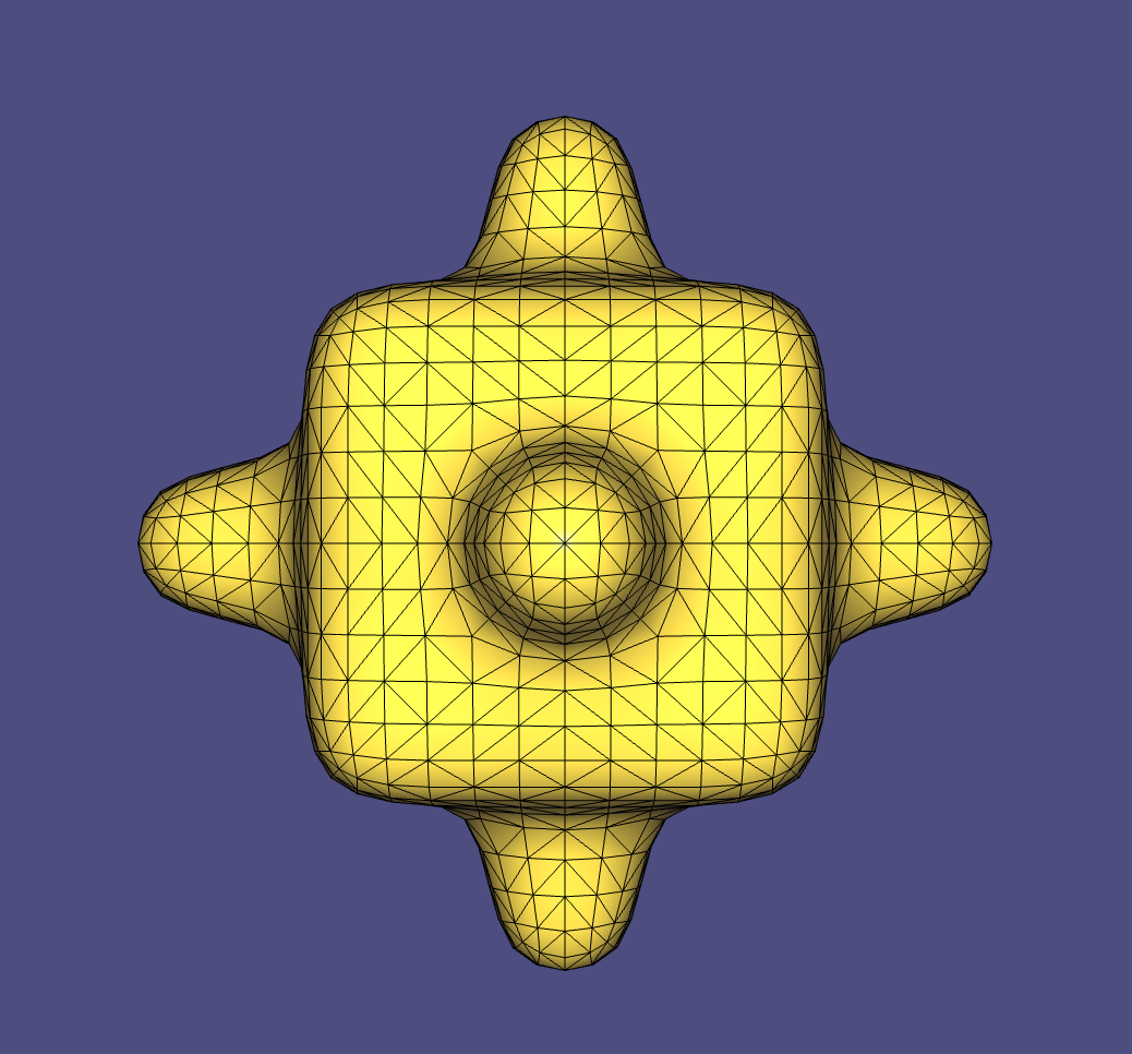
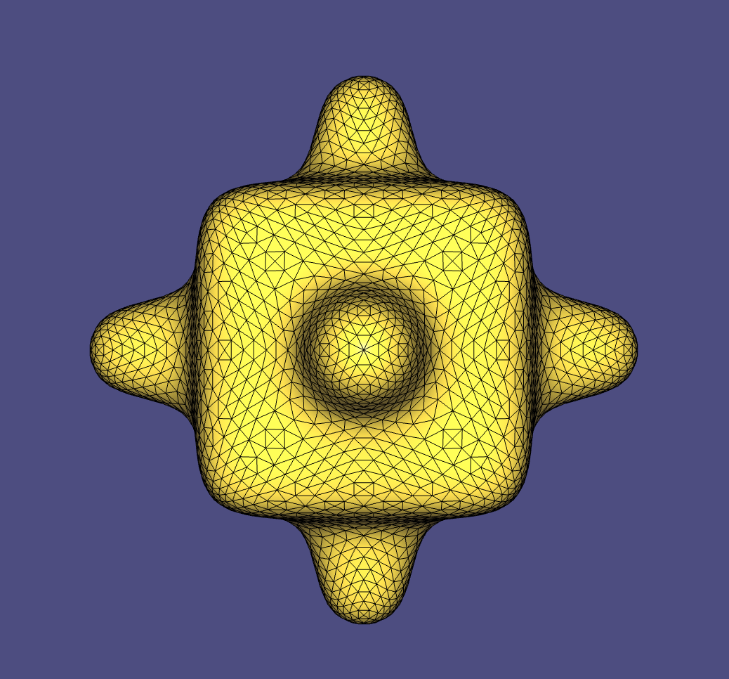
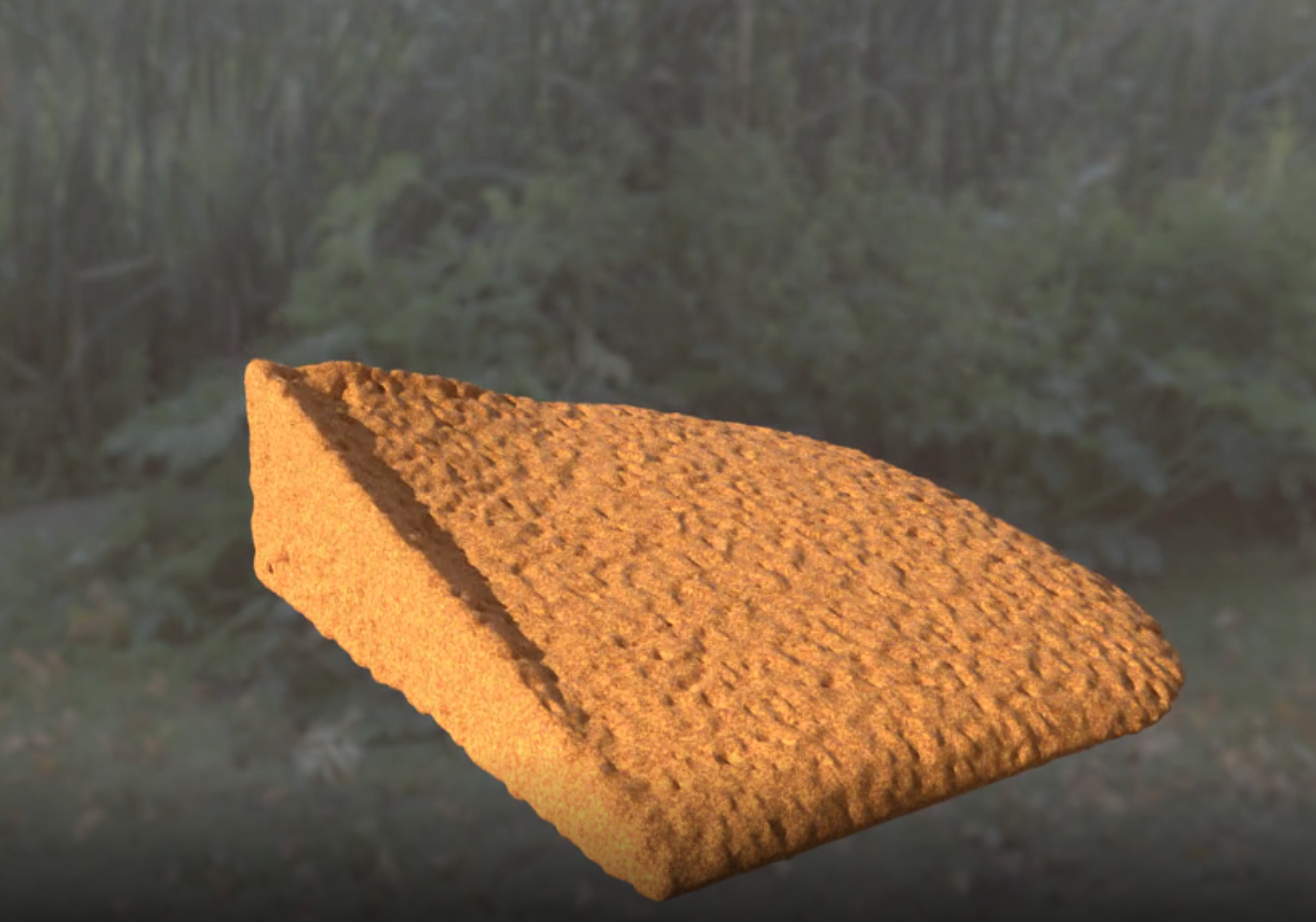
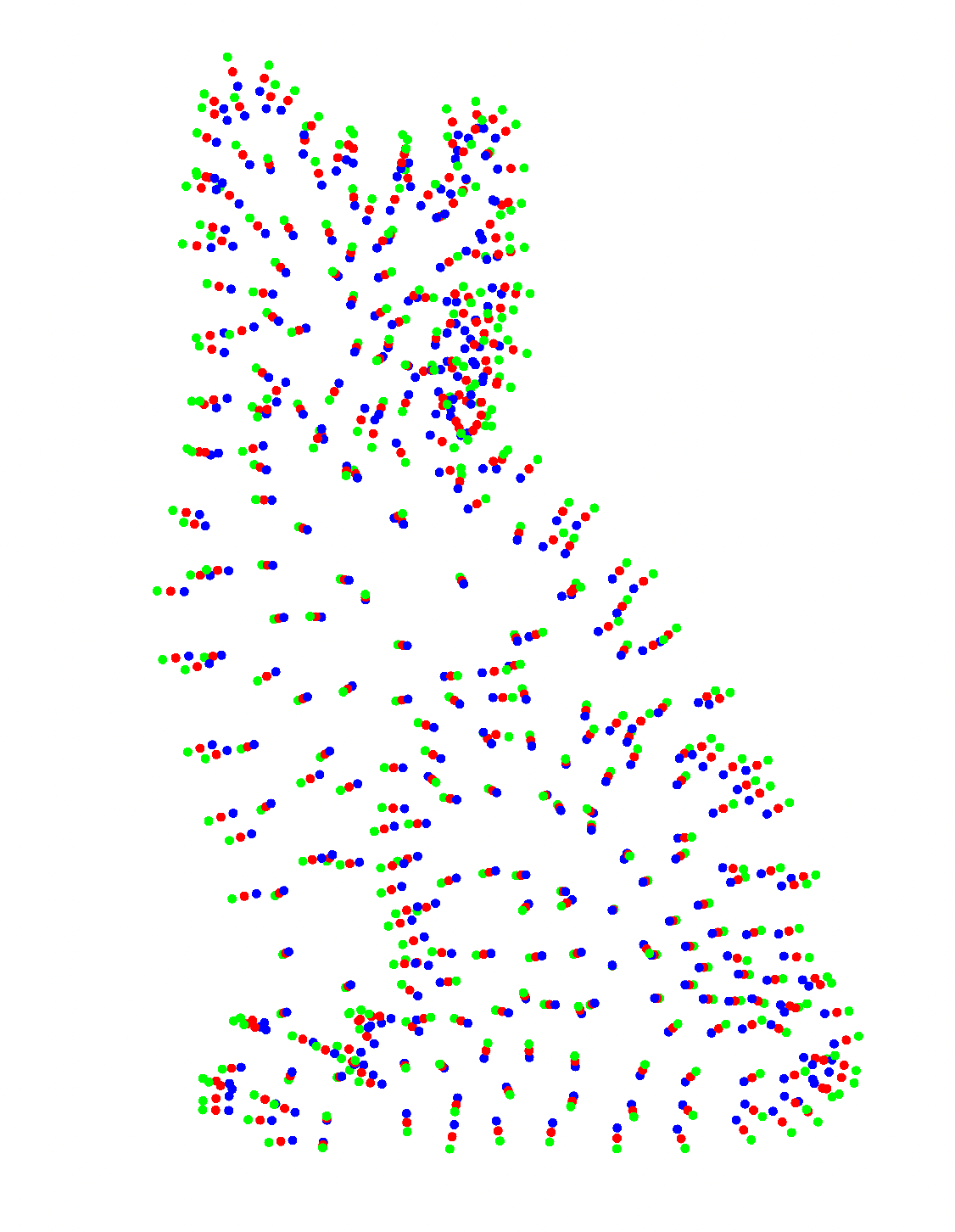
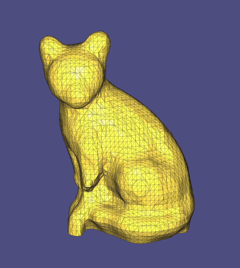
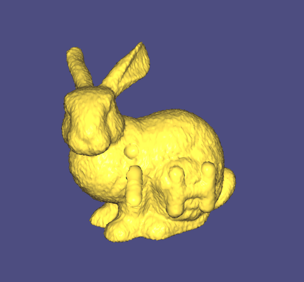
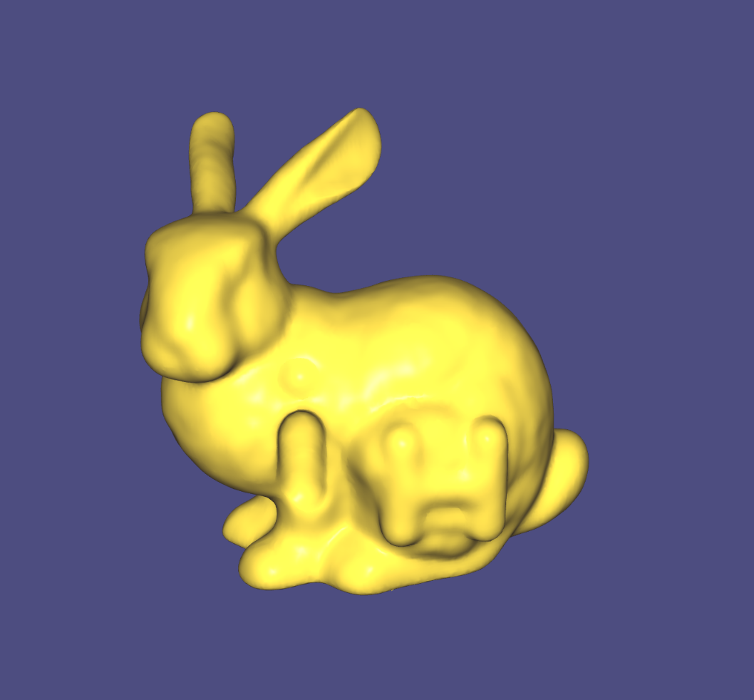
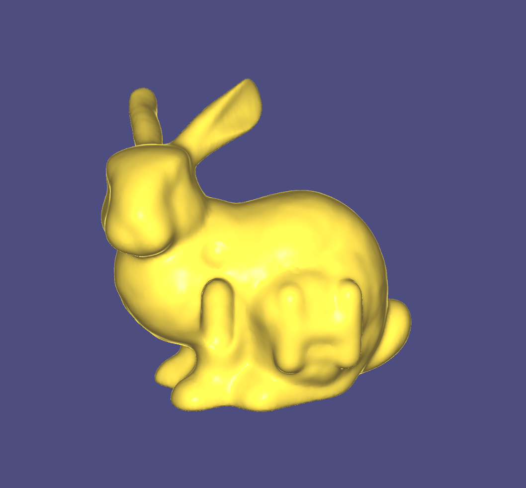
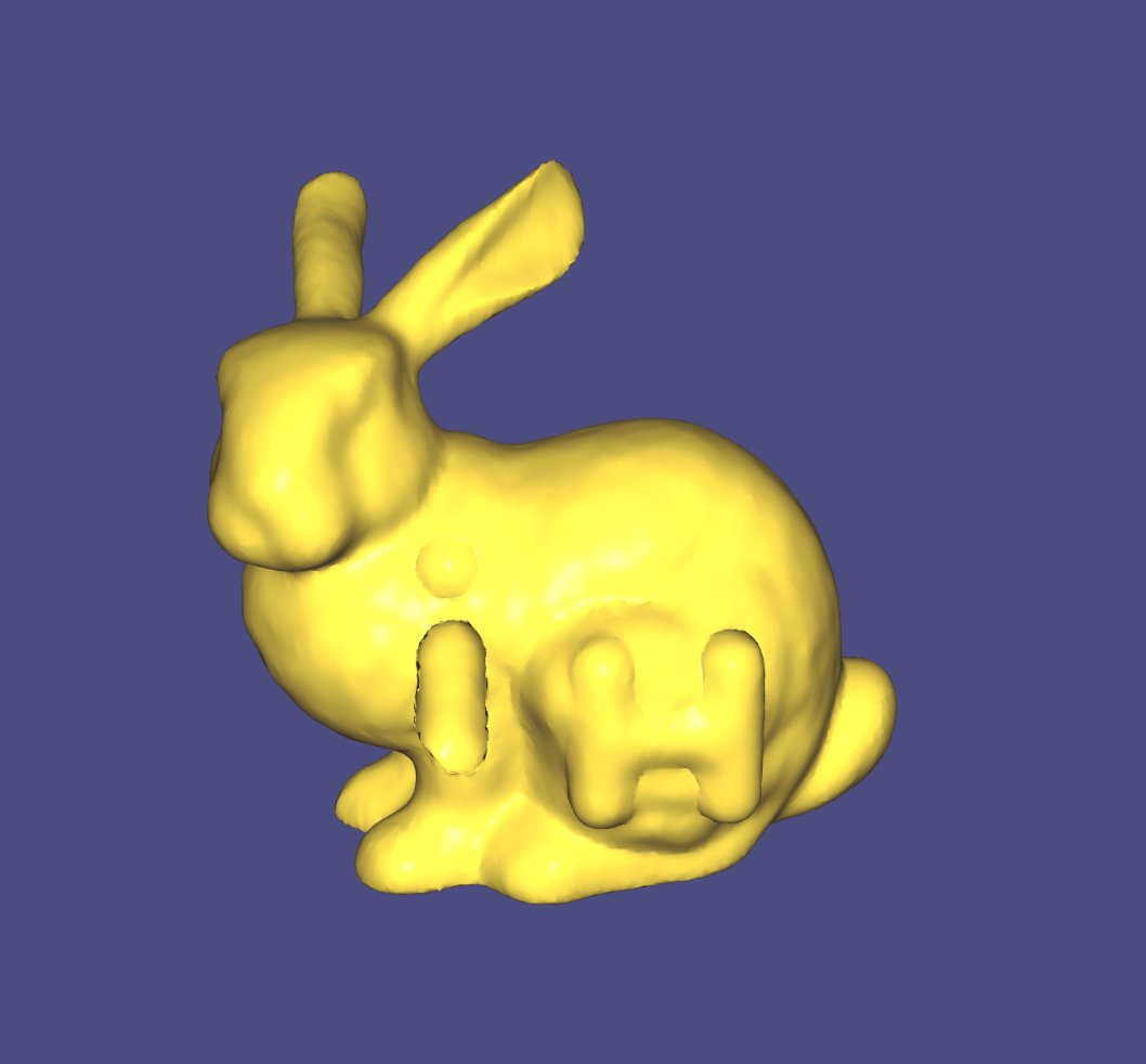
2. Implicit Surface Reconstruction
Compute an implicit function using Moving Least Square (MLS) approximating a 3D point cloud with given normals. Sample the implicit function on a 3D volumetric grid and then apply the marching cubes algorithm to extract a triangle mesh of this zero level set.
We can tune different parameters to get a better reconstruction, e.g. grid resolution, the polynomial degree of fitting, the weighting function used in MLS.
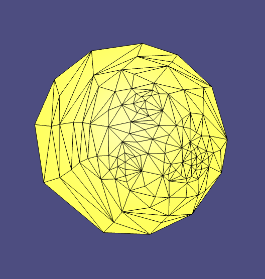
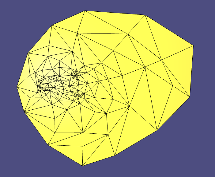
3. Mesh Smoothing
Explicit Laplacian Smoothing. typically needs more iterations and smaller step sizes to produce comparable results as the implicit method.
Implicit Laplacian Smoothing. It needs very few iterations to produce a reasonable result. The implicit method is stable with a relatively large step size.
Bilateral Laplacian Smoothing. Preserve the sharp edges better.
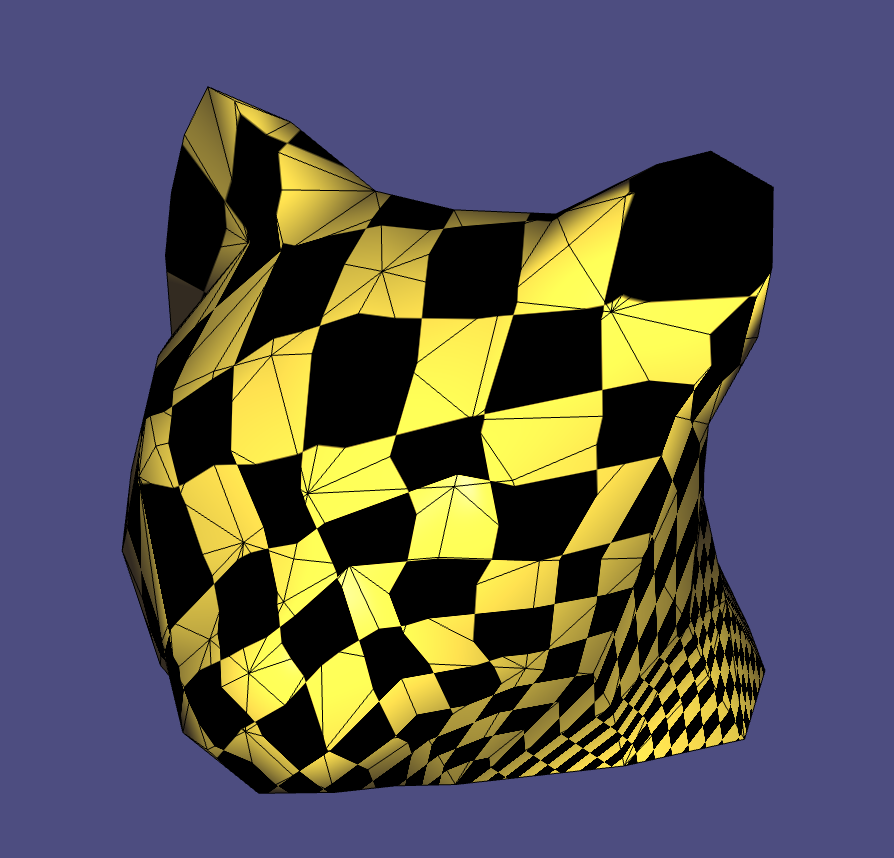
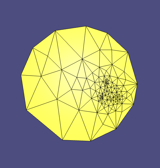
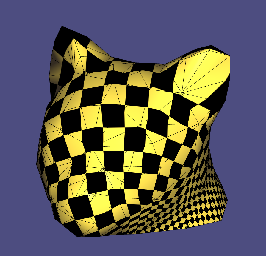
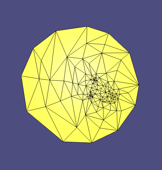
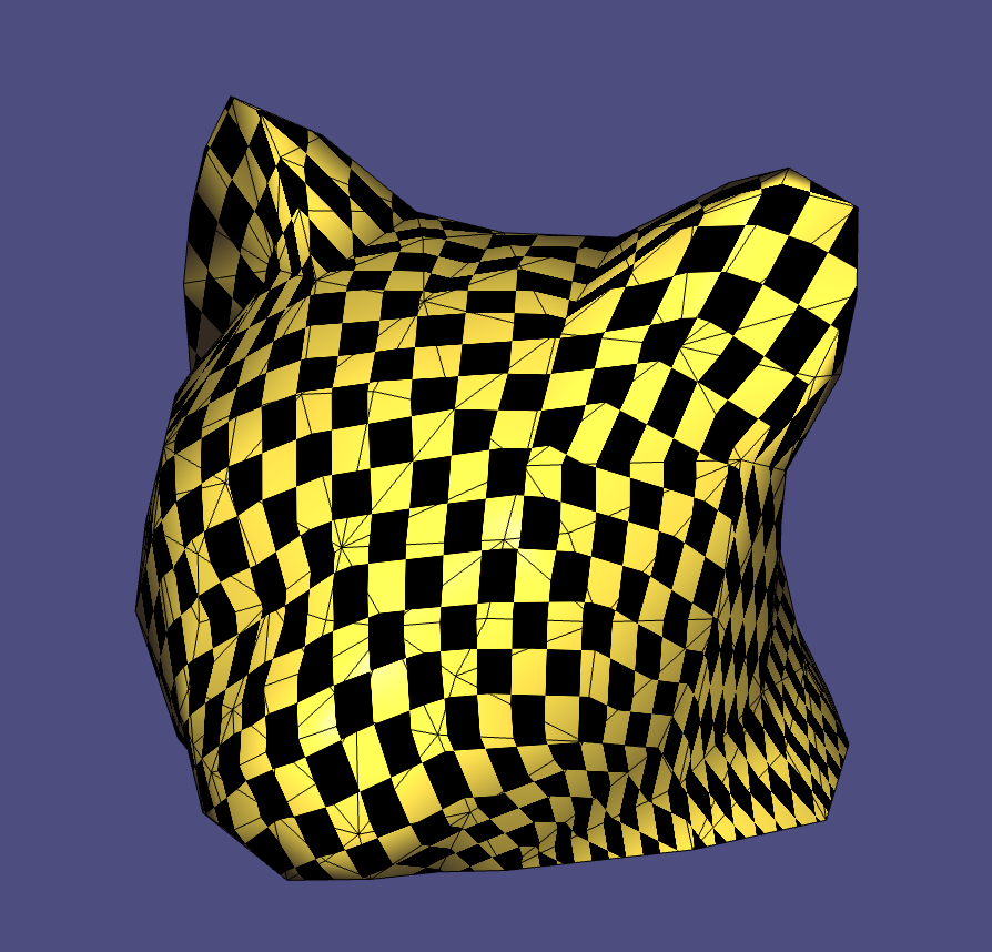
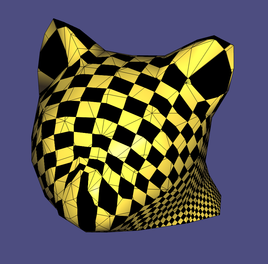
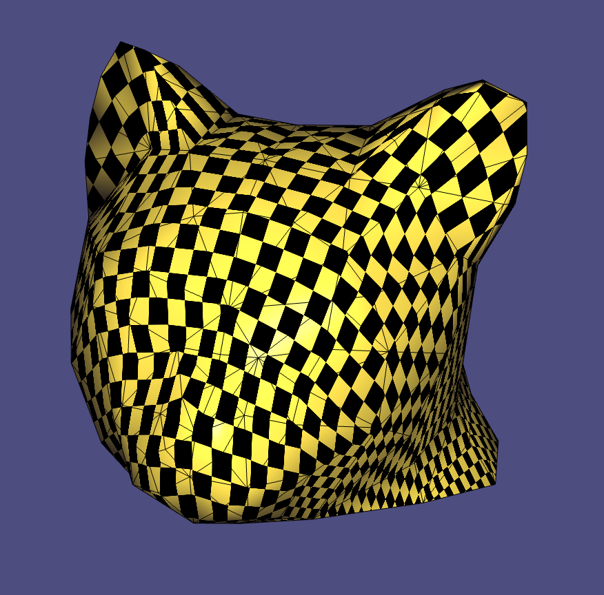
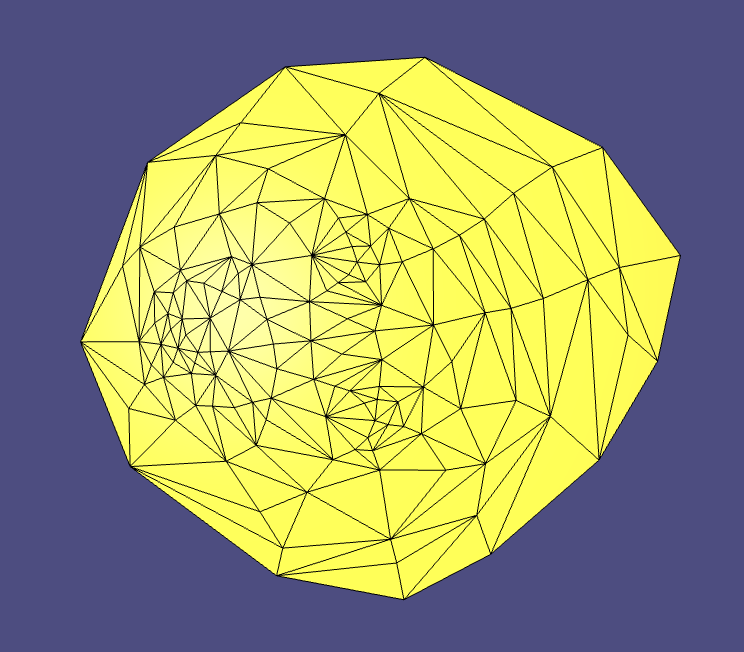
4. Mesh Parameterization
Parameterize a mesh by minimizing different distortion measures with fixed or free boundaries.
• Spring energy (uniform Laplacian)
• Dirichlet/harmonic energy (cotangent Laplacian)
• Least Squares Conformal Maps (LSCM)
• As-Rigid-As-Possible (ARAP)
Uniform (fixed boundary)
Cotangent (fixed)


LSCM (fixed)
ARAP (fixed)
LSCM (free boundary)
ARAP (free)
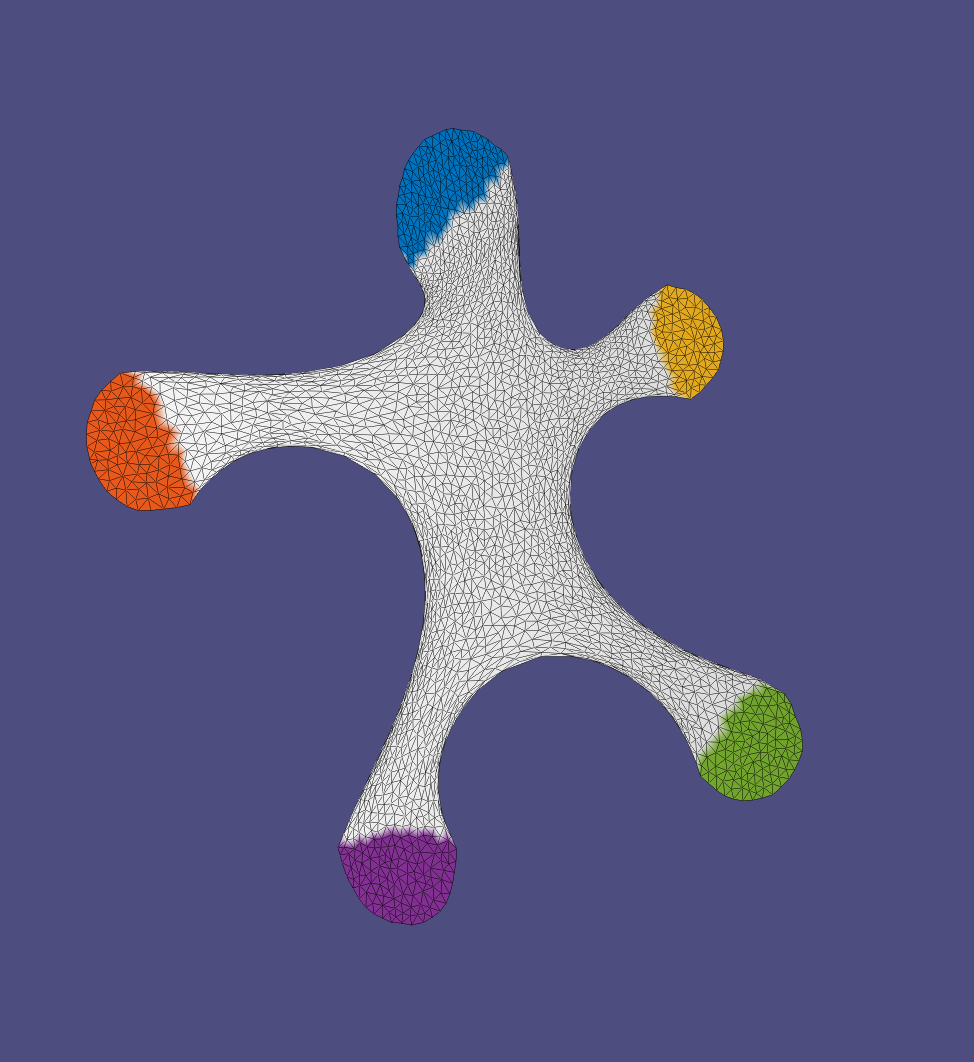
5. Shape Deformation
Multi-resolution mesh editing. The algorithm is as follows:
• Selecte the handles
• Remove high-frequency details
Original mesh -> smoothed mesh
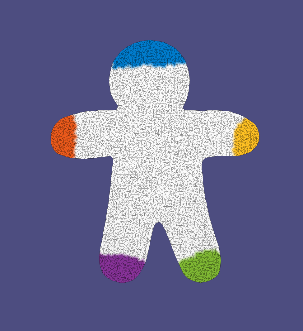
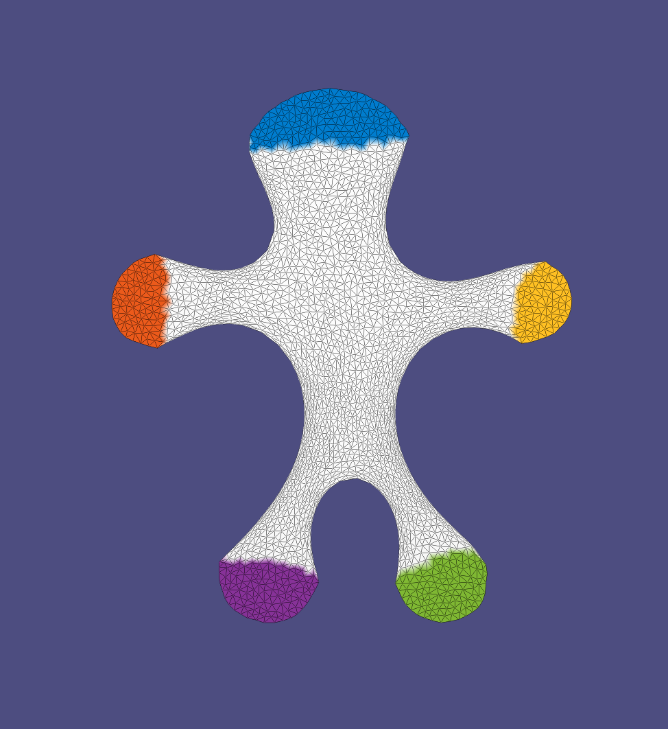
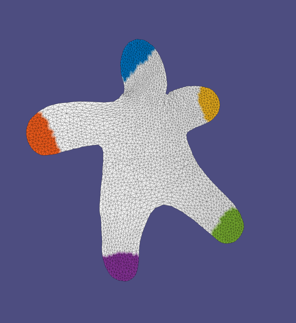
• Deform the smooth mesh
• Transfer high-frequency details to the deformed surface
Deformed smooth mesh -> deformed original mesh
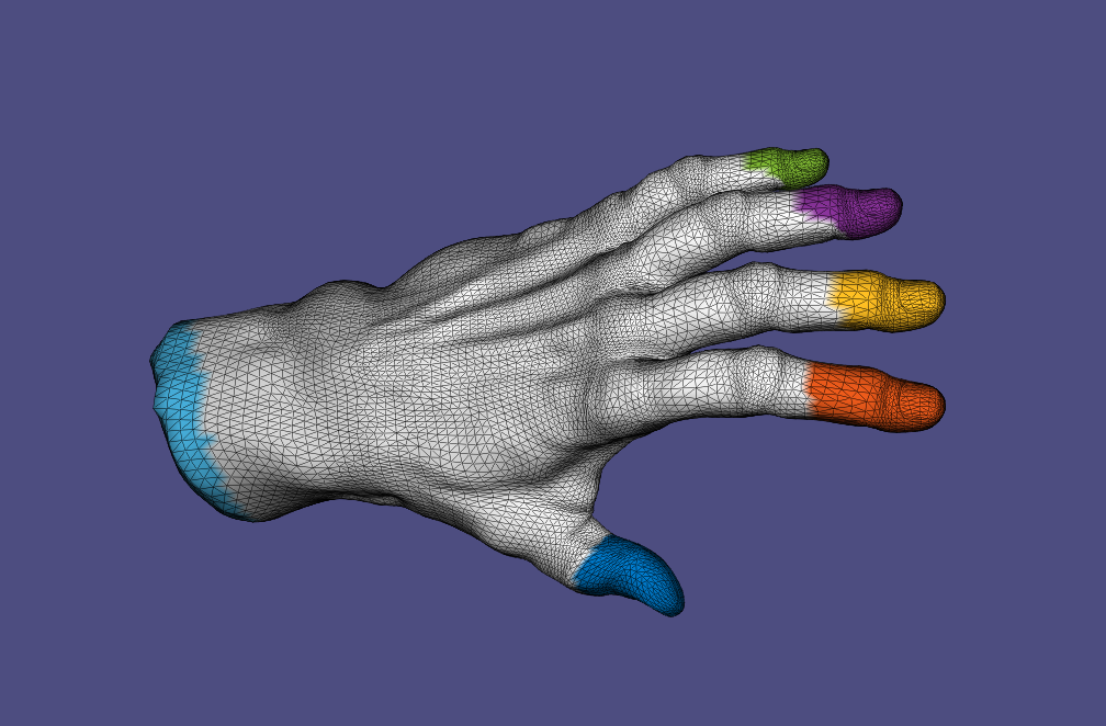
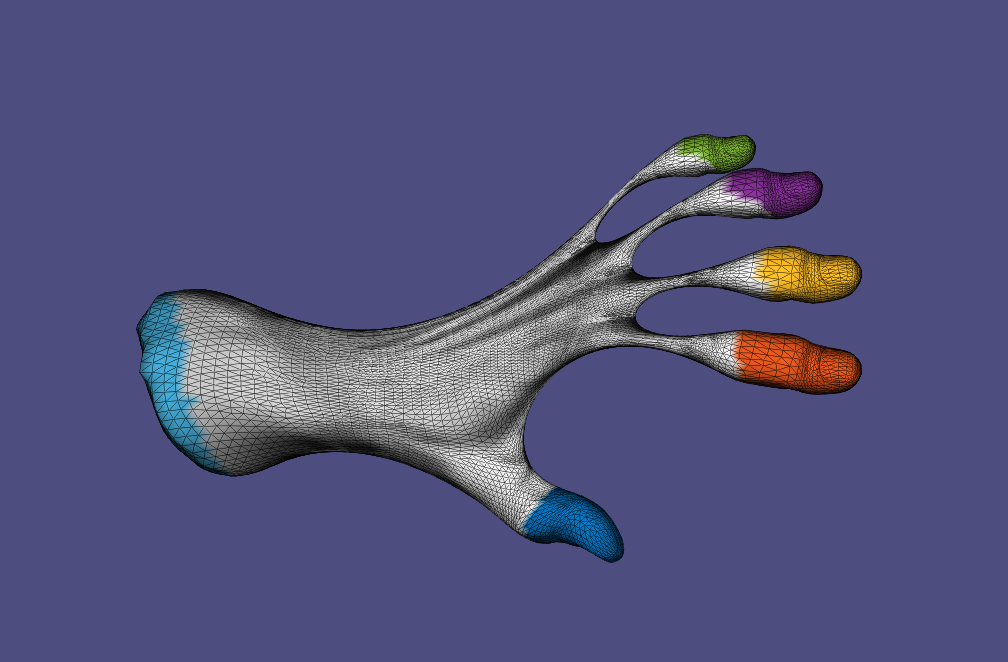
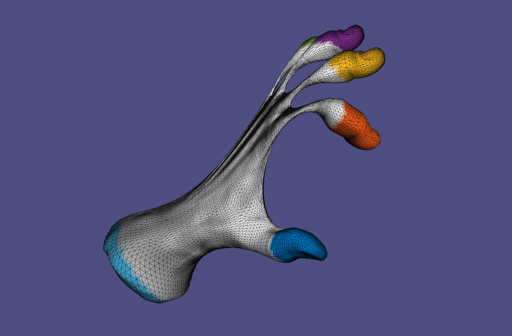
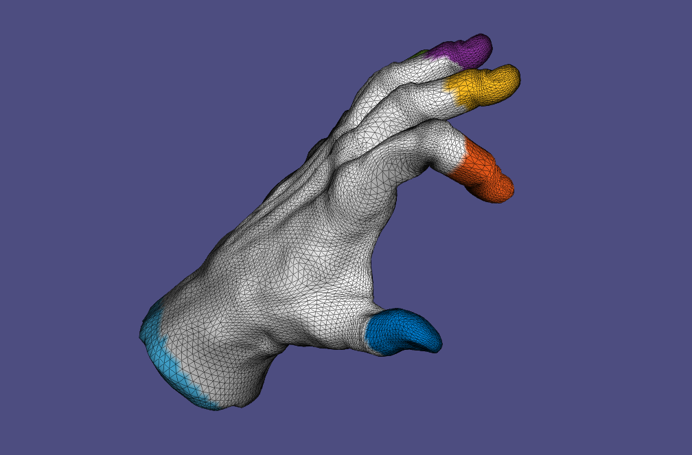
6. Skinning & Skeletal Animation
We apply skeletal deformation with
• Per-vertex Linear Blending Skinning (LBS)
• Dual Quaternion Skinning (DQS)
• Per-face Linear Blending Skinning with Poisson stitching
• Context-aware skeletal deformation, where multiple example poses are provided to improve the deformation
Accelerate Marching Cubes
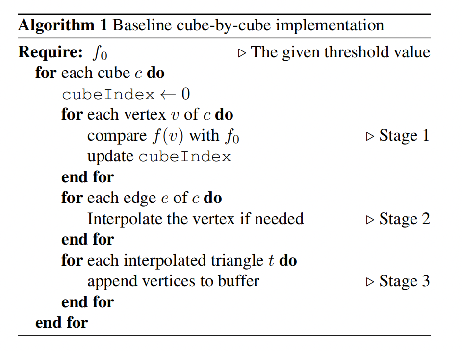
This project studies the single-core performance optimization of Marching Cubes (MC) algorithm. Given a scalar field with values discretely evaluated on a 3D grid, and a certain threshold value, the MC algorithm reconstructs the threshold isosurface as a triangle mesh. The original algorithm marches in a cube-by-cube fashion within the grid. The process can be divided into three stages: threshold comparison, vertex interpolation, and triangle assembling.
Optimization
We present an optimized implementation of the MC algorithm that marches level-by-level on the grid. It utilizes the feature of the grid structure to store, reuse, and share intermediate results in order to avoid redundant computation and allow for more memory locality.
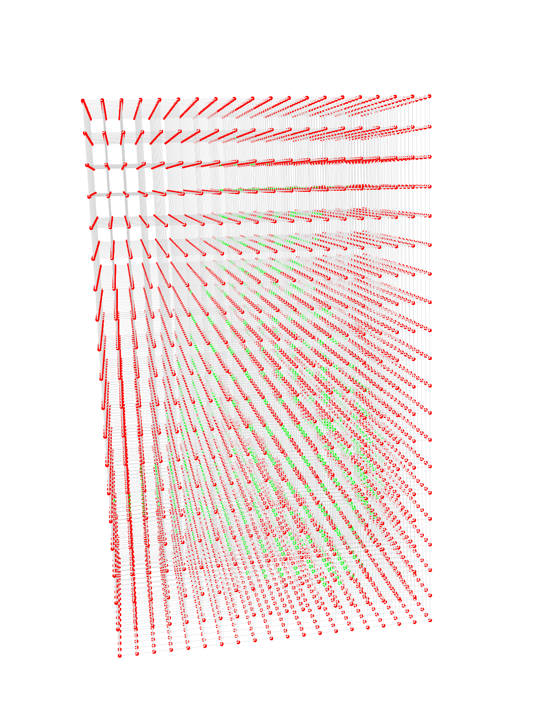
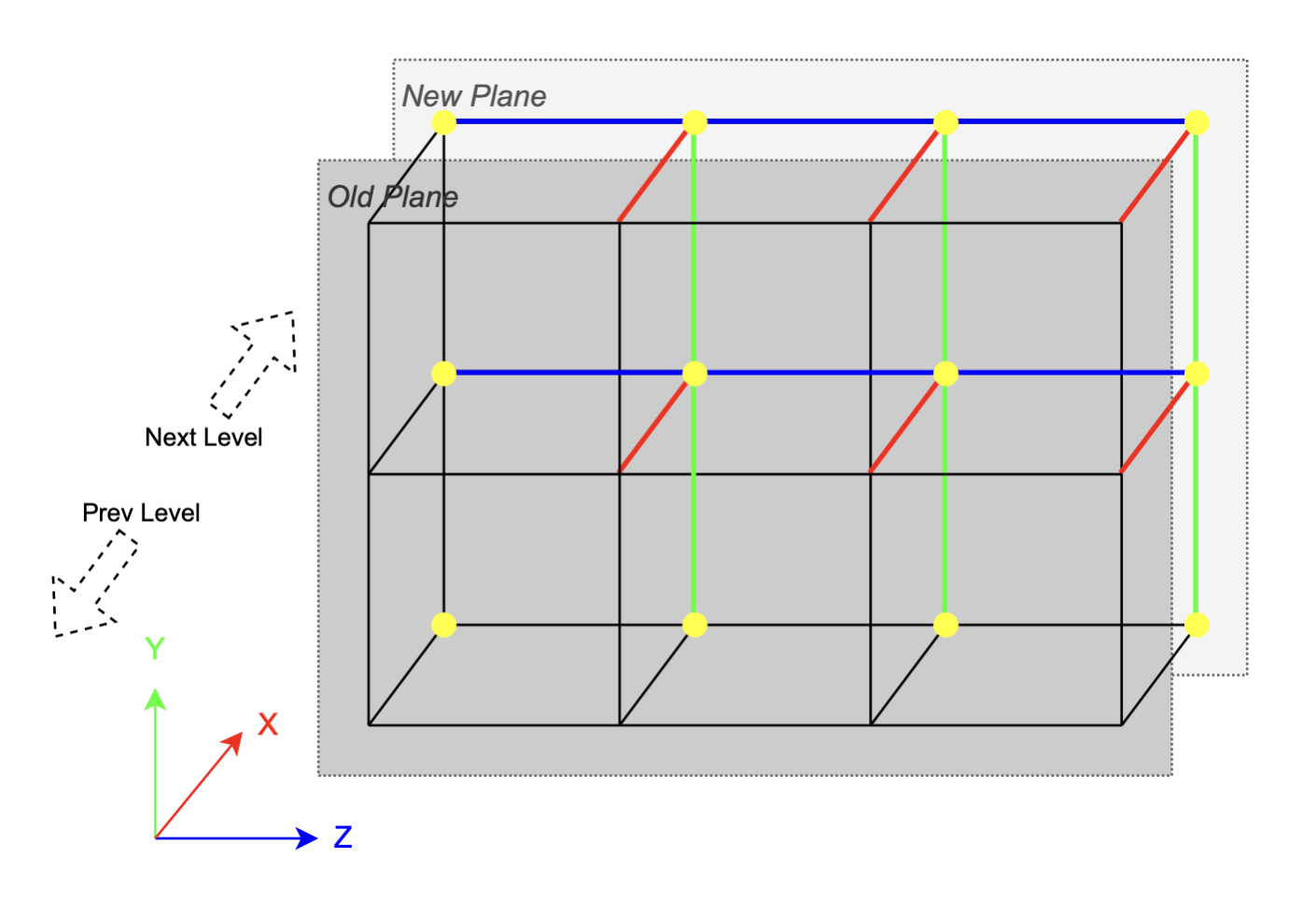
Here is an illustration of the level-by-level optimization. The current level of cubes contact with its two neighbors on two planes. When iterating over the current level, most cubes only need to do the vertex interpolation on 3 edges (colored with colors corresponding to the axes). Threshold comparison and vertex interpolation (on YZ edges) results are only written on the new plane, while the results on the old plane is inherited from previous level. Two ping-pong buffers are used, each one serves for a plane and alternate for odd and even levels. By marching through all the levels we could process all cubes without any redundancy.
During the implementation of level-by-level method, we also need to make some important optimization decisions. The first one is to use the format of indexed mesh as the output which is more compact. Each interpolated vertex position will be stored exactly once, and each triangle is identified by 3 indices. The second critical change is to replace the most costly branches needed during triangle assembling stage with arithmetic operations and look-up tables.
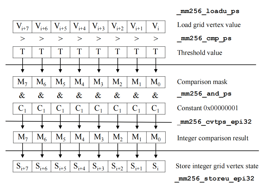
On the basis of the level-by-level method, we can integrate the SIMD vectorization into it. AVX2 intrinsics to vectorize the comparison of grid point values and the threshold, the determination of cube topology and the interpolation of new edge vertices.
Vectorization of threshold comparison
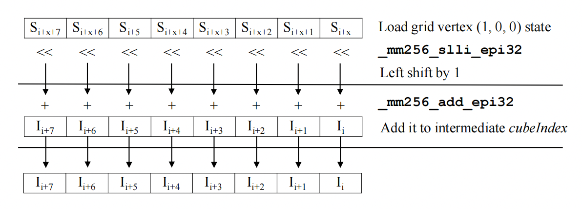
Determine cube topology based on the grid points' threshold comparison state. Here grid point at position (1, 0, 0) is used as example. We repeat this for all 8 cube vertex positions.
During vertex interpolation, not every edge intersects with the isosurface and thus needs interpolation. Therefore, we need to first determine which edges are actually intersecting the isosurface. To this end, We use a two-pass method. We categorize the edges into three different types based on which direction they are in, namely the direction of X, Y or Z axis. In the first pass, for each of the three directions, we generate a data structure telling which of the edges require interpolation, which is similar to the Compressed Sparse Rows (CSR) representation. In the second pass, we conduct the following two steps.
1. Gather start and end vertices values for vertex interpolation.
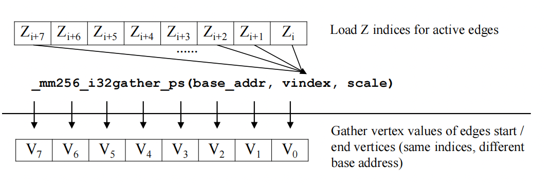
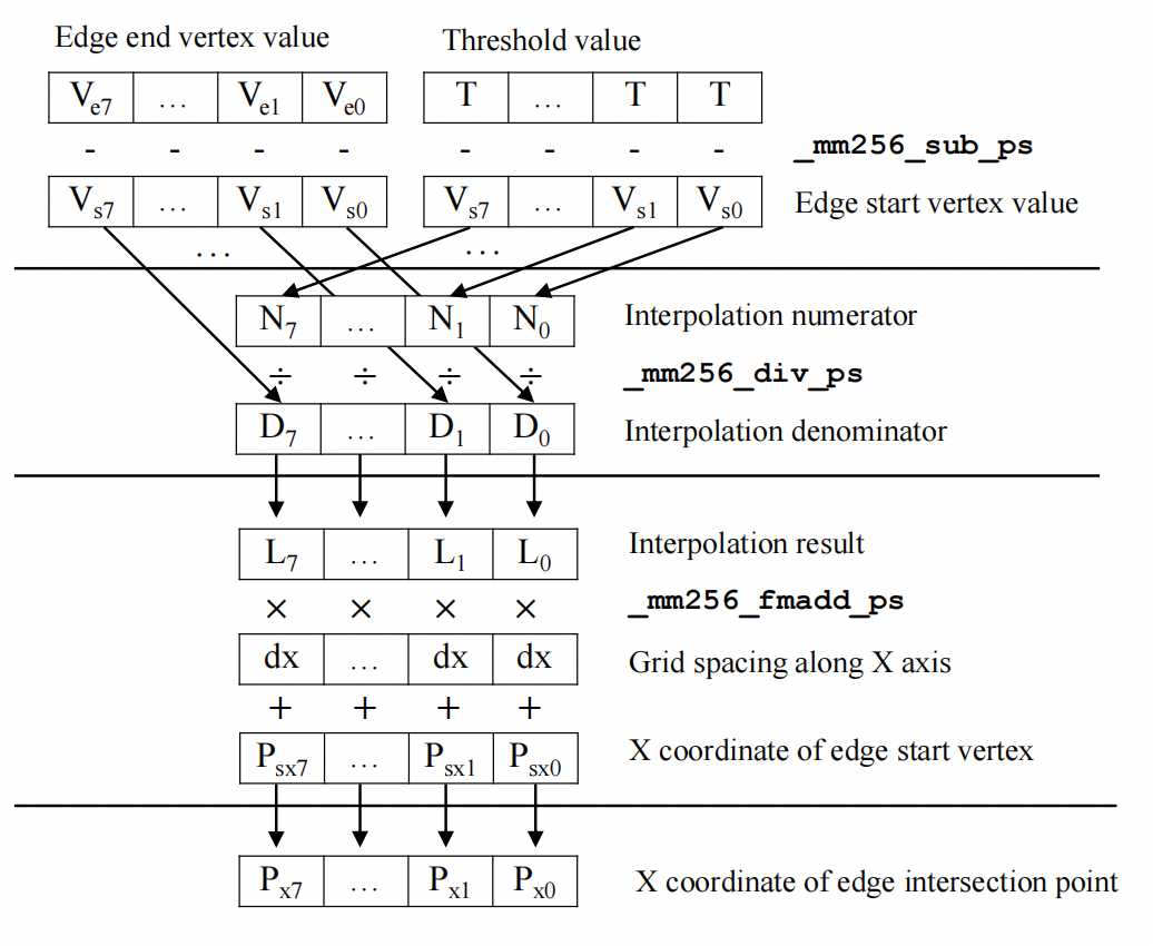
2. Vectorized calculation of edge intersection coordinates. Use the edges along X-axis as an example.
Results
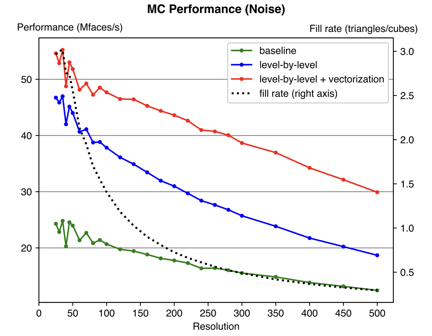
Experiment results show that our optimization could achieve 2-3x speedup compared to the naive implementation. The optimization proposed is general and should be effective for any resolution and specific values of the input data. The fixed cost of the algorithm depends on the number of cubes, while the variable cost depends on the number of triangles generated. Thus, we also plot the “fill rate” in the figure (value on right axis), which is defined as the ratio of the number of triangles to the number of cubes (resolution cubed).
Performance plot for a random scalar field generated using Perlin Noise as input. It is continuous but changes quickly due to the high frequency, thus the isosurface intersects with many cubes.
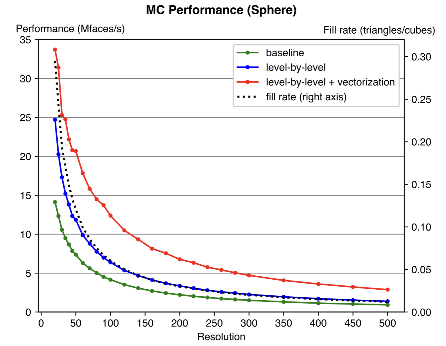
Performance plot a SDF field to a sphere as input. This is a sparse example and most cubes are empty.
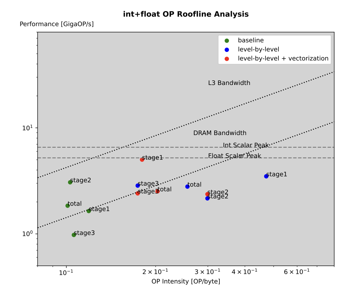
Roofline analysis. We can see the improvement on operational intensity compared to the baseline. This is mainly because the level-by-level strategy reduces memory access of the redundant computation. The vectorization mainly happens in the first stage, and its performance gain could be clearly spotted in the plot.
The first bottleneck lies in the vertex interpolation stage. We need to decide which edges are intersecting with the isosurface using “if” statements, increase a global counter of vertex indices which is strictly order-dependent and then store it to the corresponding intermediate array. The “if” branches cannot be predicted, and ILP is difficult to increase with loop unrolling because of the global counter. The cost of actual interpolation is trivial compared to the overhead of branches and the computing and storing of the vertex indices.
The second bottleneck is in triangle assembling, where a triple level loop over the YZ axis and then over triangle table entries runs slowly. The access pattern is not consecutive in memory and can't benefit from vectorization. As the roofline plot shows, we think this bottleneck is the memory.
Conclusion
Our optimized implementation of the MC algorithm is settled on two pillars: reorganizing the structure of the computation, and using SIMD intrinsics to integrate vectorization. The proposed optimizations produce 2-3x performance gain. The strategies are general, could be used for any data and input sizes, and are possible to be integrated with other optimization techniques, such as multi-processor parallelism and spatial data structure based methods. In the future, we would like to explore the potential ways for further optimizing the current bottlenecks of our implementation, e.g., ways to increase ILP and branching efficiency in the second stage and improve memory access in the third stage.
Simulate Sand as Fluids
In this project we implement three classic hybrid fluid simualtion methods: Particle-in-Cell (PIC), Fluid-Implicit-Particle (FLIP), Affine Particle-In-Cell (APIC). These methods are called hybird as they combine the grid-based pressure solving and particle-based advection. Then based on this paper (which is also the paper introduces PIC), we implement the animation of sand based on the simulation of fluids.
For sand simulation, first we need to evaluate strain rate tensors in grid cells, which is then used to calculate and determine whether the sand cell will flow or move as rigid bodies based on the Mohr-Coulomb yield condition. Then separately simulate rigid body groups using rigid body motions, and flowing sand motions. Finally the friction condition between sand and boundaries is enforced.
The implementation is written in Taichi, a high-performance parallel language wrapped in python. This is an open-source project and has received 50+ stars.
Github Page
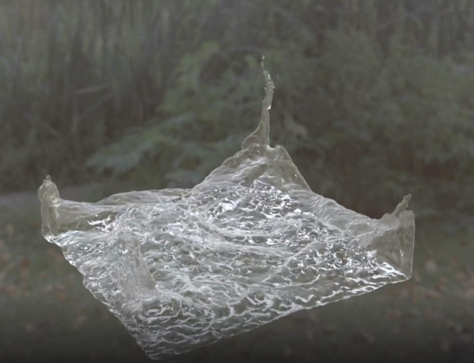
Rendered results
APIC fluids
APIC sand