Volumetric Path Tracer

"The toys invasion"

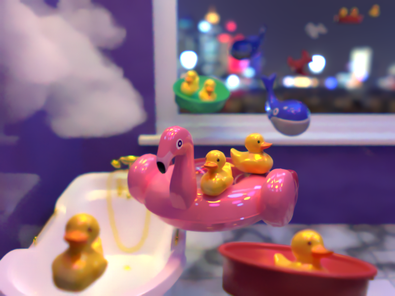
This work is among the three "Honorable Mention" prizes in ETH 2022 CG rendering competition.

Images as Textures
Textured Area Emitter
Procedural Textures
Normal Mapping
Heterogeneous Volumetric Participating Media
Anisotropic Phase Function
Procedural Volumes

Images as Textures

We have two types of image textures, one for .exr and the other for other common image formats (e.g. png and jpg). Exr format is supported through Nori's bitmap reader. Other common image formats like .png and .jpg are supported by the stb_image library. The two textures implement the eval method with bilinear filtering. For the sRGB color textures, we apply gamma correction to convert the colors to linear space.

Here is an example of image texture. The original texture:

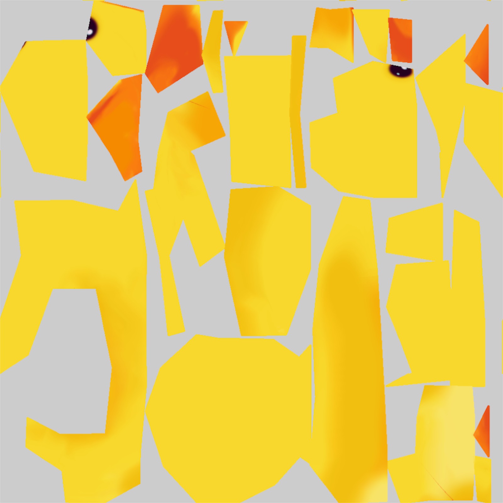
The textured mesh with 512 spp:

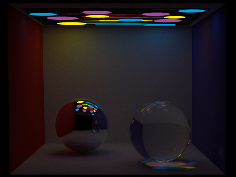
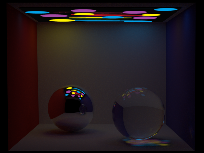
Textured Area Emitter

Here is an example of a textured area emitter.

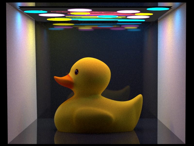
In Mitsuba, it is not possible to specify the emitter radiance and the emitter texture at the same time. In other words, radiance is decided only by the image value. If we set the radiance in our system to (1, 1, 1), we can make a comparison. (spp = 512)

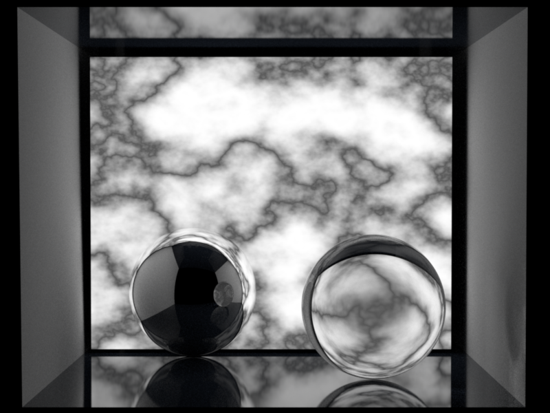
Procedural Textures

For the procedurally generated texture, we choose to implement the marble texture. We used [1] as a reference. It is based on the classic Perlin noise. To create the pattern of the marble, we use several octaves of Perlin noise to form the fractional Brownian motion. Each time we reduce the weight by multiplying the persistence, doubling the noise frequency, and finally applying a cosine function to it.

Validation

Here is the generated texture (also used as a textured area emitter, spp=512):

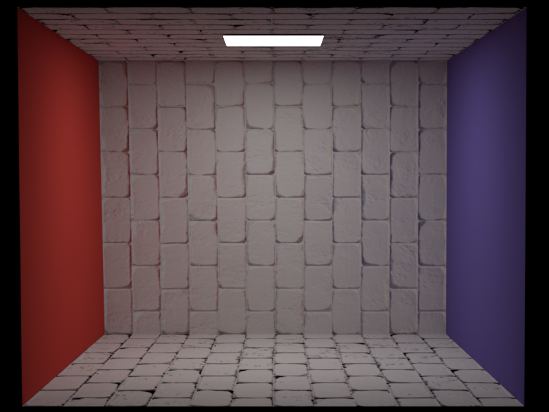
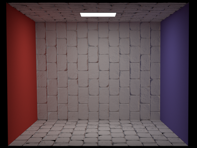
Normal mapping

During the querying of the shading frame when setting up the intersection, we use the shape uv to evaluate the normal map. Then the calculated normal is used to create the shading frame instead of using the geometric frame or the mesh normals. We need to compute the tangent and bitangent to create the tangent space coordinates and convert the normal to world space properly.

Validation

The validation is a comparison to Mitsuba's normal map. (spp=512)

Volumetric Participating Media

We have two types of volume, one is a constant volume (homogeneous) and the other is a grid volume (heterogeneous). For each volume, we can specify a volume AABB bounding box, the absorption and scattering coefficients, and the phase function. The volume class should implement two methods: (1) sample the free flight distance and (2) compute the transmittance. The transmittance is computed with ratio tracking, which is similar to the implementation of PBRT v3 [3]

Constant volume / Homogeneous

For the homogeneous medium, the absorption and scattering coefficients sigma_a and sigma_s are constant throughout the bounding volume.

Grid volume / Heterogeneous

We can either load from Mitsuba .vol single-channel density file or use the procedurally generated density field. A density grid is created and we evaluate the density for a position using the trilinear interpolation. If the density is procedurally generated, we provide some parameters to tweak the density field. The main difference between the homogeneous and heterogeneous volume is that we consider different extinction coefficients for different volume density.

Volumetric path tracer with MIS

We implement a volumetric path tracer with the MIS technique. When we trace a ray, we sample the free flight distance according to all the scene media to check whether there is an interaction within the medium. If there is an interaction, we start a new ray from the place of interaction which is decided by the free flight distance. Otherwise, we will continue the ray to see if it intersects with the scene or not.

To reduce noise, we add light sampling for each medium-interaction/scene-intersection and apply balanced heuristics to compute the MIS weights. For each light sampling, we include the influence of the medium through the transmittance along the shadow ray. The material pdf is from the phase function for a medium interaction, or from BSDF for a surface intersection.

Validation

To validate the implementation, we have the results compared to the rendering of Mitsuba 3. The Mitsuba results are rendered with the volumetric path tracer, with a low discrepancy sampler and 1024 spp.

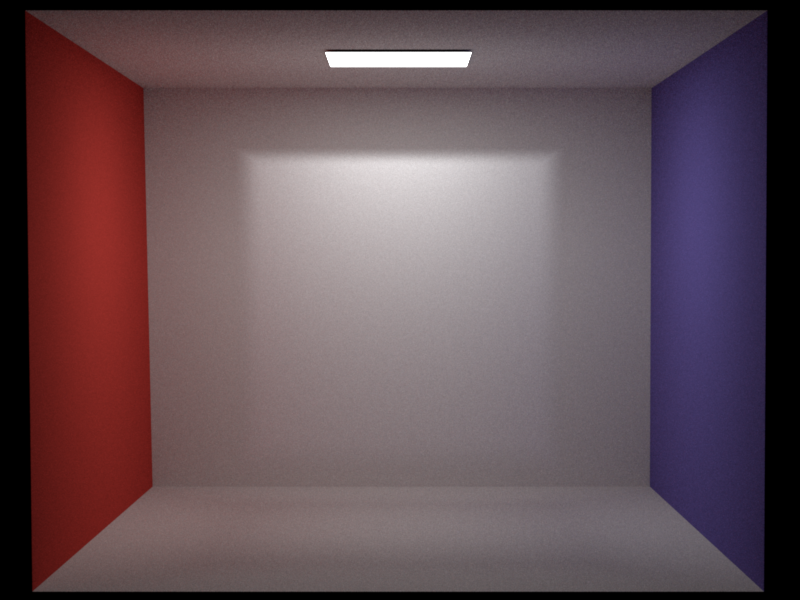
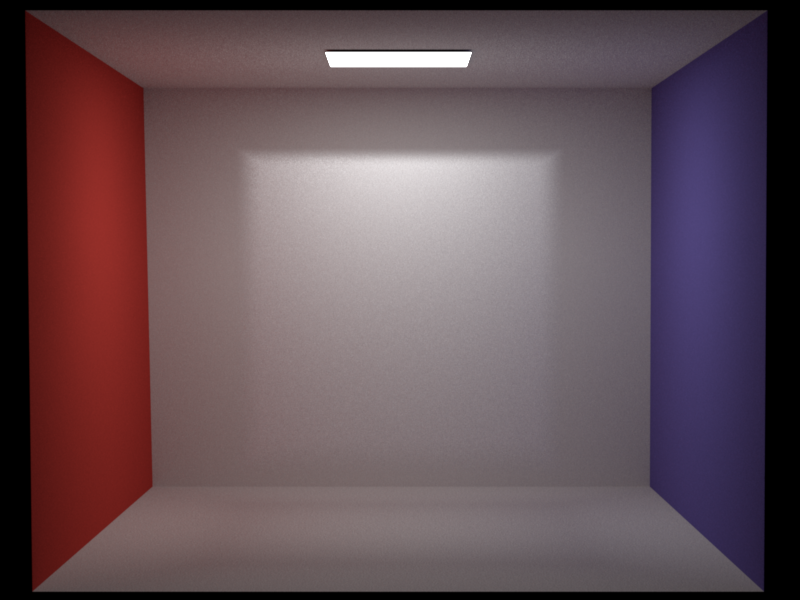
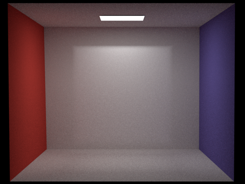
Here is the validation of a homogeneous volume (sigma_a = (0, 0, 0), sigma_s = (1, 1, 1), spp = 512):

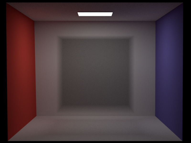
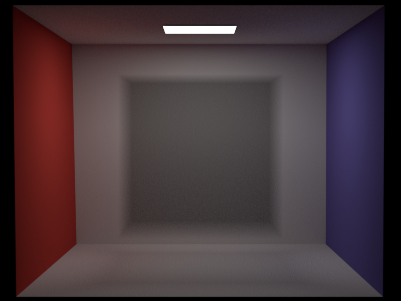
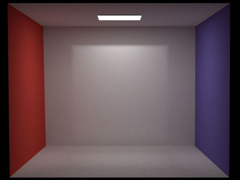
The effect of pure absorption (sigma_a = (1, 1, 1), sigma_s = (0, 0, 0), spp = 512)

Here is an example of more than one volume (sigma_a = (0, 0, 0), sigma_s = (1, 1, 1), spp = 512):

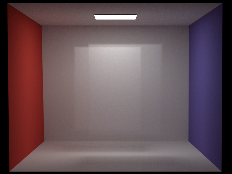
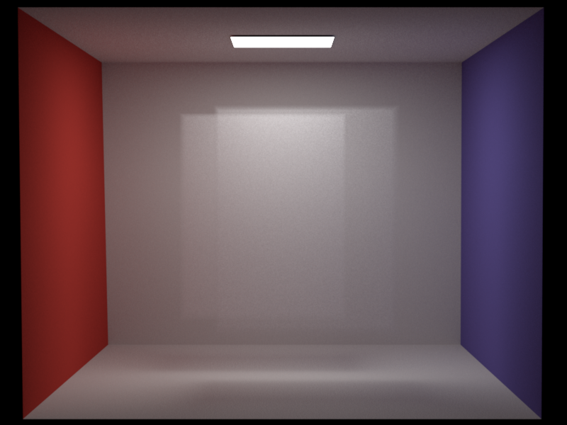
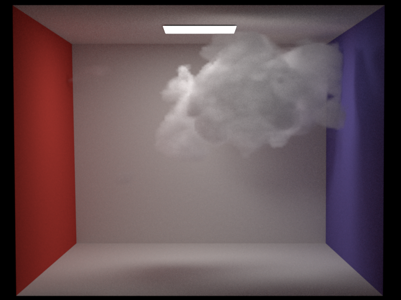
Here is the validation of a heterogeneous volume (sigma_a = (0, 0, 0), sigma_s = (10, 10, 10), spp = 512). The density is loaded from smoke.vol file from Mitsuba website:.

Anisotropic Phase Function

For the anisotropic phase function, we implement the Henyey-Greenstein phase function. The phase function will be added as a child of a volume. During a medium interaction, we can sample the next ray according to phase function based on the original ray direction. During the light sampling, we can evaluate the pdf based on the ray direction and the direction toward the light.

Validation

Here is an example of HG phase function: (sigma_a = (0, 0, 0), sigma_s = (1, 1, 1), g = 0.7, spp = 512):

Procedural Volume

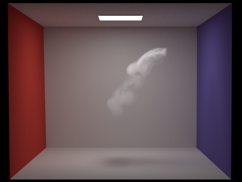
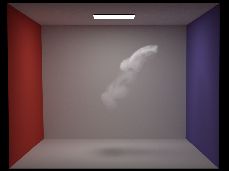
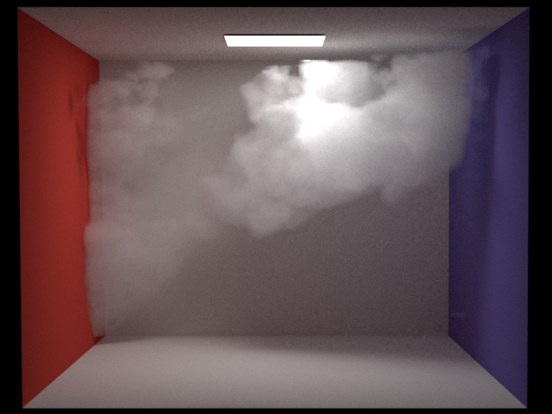
Procedural volume is used to generate the density field of clouds. We choose the Worley noise, a variant of Voronoi noise, which is suitable to generate the base shape and details of clouds. The reference for the implementation is given by [2]. Again, we use several octaves to generate the fBm noise. We first create a base-shape-noise and use a threshold to keep the high-density part; Then we create a detail-noise with higher frequency components of Worley noise. By subtracting the detail-noise from the base-shape-noise, we get a cloud-density field with good details. To avoid the sudden clamp around the boundaries, we apply attenuation to the density close to the boundaries.

Here are some generated density fields (grid resolution = (128, 128, 128), sigma_a = (1, 1, 1), sigma_s = (20, 20, 20), g = 0.1, spp = 512):

References

[1] Texture noise. PBRT Book 3rd. https://www.pbr-book.org/3ed-2018/Texture/Noise
[2] Nubis: Authoring Real-Time Volumetric Cloudscapes with the Decima Engine https://advances.realtimerendering.com/s2017/index.html/
[3] Volumetric light transport. PBRT Book 3rd. https://www.pbr-book.org/3ed-2018/Light_Transport_II_Volume_Rendering/Volumetric_Light_Transport